|
Canoe
Comprehensive Atmosphere N' Ocean Engine
|
|
Canoe
Comprehensive Atmosphere N' Ocean Engine
|
This example shows the simulation of a sinking air bubble in two dimensions. It is proposed by [2] for benchmarking the numerical methods. The temperature anomaly of the cold air bubble is described by:
\begin{equation*} \Delta T = -15\;\text{K} \frac{\cos(\pi L)+1}{2}, \quad L < 1, \end{equation*}
where \(L\) is the normalized distance to the center of the cold air bubble at \((x_c,z_c)\).
\begin{equation*} L = \Big(\big(\frac{x - x_c}{x_r}\big)^2+\big(\frac{z - z_c}{z_r}\big)^2\Big)^{1/2}. \end{equation*}
Particularly, \(x_c=0\) km, \(z_c=3\) km, \(x_r=4\) km and \(z_r=2\) km. The domain is two-dimensional and is 6.4 km tall and 25.6 km wide. Either the horizontal or the vertical resolution is 100 m. The background atmosphere is isentropic, where the temperature is 300 K at 1 bar surface pressure. Initially, the bubble is aloft in the air, hydrostatically balanced. Convective instability causes the bubble to sink while trigging horizontal and vertical velocity fields. The resulting density current propagates out at the surface developing Kelvin-Helmholtz instability. The purpose of the program is to resolve the instability and calculate the evolution of the density current.
Since this example is the first of the series. We would spend a few paragraphs on how to configure, compile and run the code. The first step of running the code is to patch the code. The Canoe model is developed based on the Athena++ project. We have modified many source codes and have added support for atmospheric simulation. In order to keep track of our modifications and keep it seperate from the main stream development of the Athena++ code, all source files that are in conflict with the original Athena++ code are placed in a dedicated folder drum. Then we patch the code using a python script:
After this script was executed, a file named patch_files will appear containing replacement files and supplementary files. Then the program will configure according to the rules specified by the patch_files.
Next, configure the program using the following command.
straka is the name of the application. Internally, the configure script searches for file named straka.cpp under the directory src/pgen. It is the problem generator file that will be complied in the next section. 3 is the number of grids in the ghost cells outside of the computational domain. A higher order numerical scheme requires a larger number of ghost cells. We are using the Weighted Essentially Non-Oscillatory (WENO) method, which requires 3 ghost celss. Lastly, we enable the NetCDF output by the option -netcdf. If successful, a messge will appear saying:
Your Athena++ distribution has now been configured with the following options:
  Problem generator:          straka
  Coordinate system:          cartesian
  X1 Grid ratio:              1.0
  Equation of state:          adiabatic
  Ammonia vapor id:           -1
  Water vapor id:             -1
  Riemann solver:             hllc
  Chemistry:                  chemistry
  Forcing Jacobian:           JacobianGravityCoriolis
  Magnetic fields:            OFF
  Number of vapors:           0
  Number of phases:           1
  Number of scalars:          0
  Special relativity:         OFF
  General relativity:         OFF
  Frame transformations:      OFF
  Self-Gravity:               OFF
  Super-Time-Stepping:        OFF
  Shearing Box BCs:           OFF
  Debug level:                0
  Code coverage flags:        OFF
  Linker flags:               -Lsrc/math -lclimath -lnetcdf
  Floating-point precision:   double
  Number of ghost cells:      3
  MPI parallelism:            OFF
  OpenMP parallelism:         OFF
  FFT:                        OFF
  HDF5 output:                OFF
  NETCDF output:              ON
  PNETCDF output:             OFF
  Compiler:                   g++
  Compilation command:        g++  -O3 -std=c++11
Then we compile the program by:
It is possible to speed up the compilation using multiple core available to the computer. To do it, we use:
in which the option -j4 suggests that using 4 cores to compile the program simultaneously. If the compilation is successfull, an executable file named "straka.ex" will appear in the bin folder.
Change directory to the running directory
It is recommended to make a soft link of the executable file to the running directory:
so that everything can be perfrom under the running directory. Finally, execute the program by
The straka.inp is the input file and the log file for the run is log.straka. The & symbol at the end lets the program to run in the background so that you can do other things. When the program finishes, many .nc files will appear. They record the dynamic fields at specified output frequency in the input file. The next step is to combine them into a single one. This functionality is provided by the script combine.py located in the root directory.
Now you will have a single output named straka-test-main.nc. Use the following command to check out the fields stored in the netcdf file :
The output is:
netcdf output {
dimensions:
    time = UNLIMITED ; // (4 currently)
    x1 = 64 ;
    x1f = 65 ;
    x2 = 256 ;
    x2f = 257 ;
    x3 = 1 ;
variables:
    float time(time) ;
        time:axis = "T" ;
        time:units = "s" ;
    float x1(x1) ;
        x1:axis = "Z" ;
        x1:units = "m" ;
    float x1f(x1f) ;
    float x2(x2) ;
        x2:axis = "Y" ;
        x2:units = "m" ;
    float x2f(x2f) ;
    float x3(x3) ;
        x3:axis = "X" ;
        x3:units = "m" ;
    float rho(time, x1, x2, x3) ;
        rho:units = "kg/m^3" ;
        rho:long_name = "density" ;
    float press(time, x1, x2, x3) ;
        press:units = "pa" ;
        press:long_name = "pressure" ;
    float vel1(time, x1, x2, x3) ;
        vel1:units = "m/s" ;
        vel1:long_name = "velocity" ;
    float vel2(time, x1, x2, x3) ;
        vel2:units = "m/s" ;
        vel2:long_name = "velocity" ;
    float vel3(time, x1, x2, x3) ;
        vel3:units = "m/s" ;
        vel3:long_name = "velocity" ;
    float temp(time, x1, x2, x3) ;
        temp:units = "K" ;
        temp:long_name = "temperature" ;
    float theta(time, x1, x2, x3) ;
        theta:units = "K" ;
        theta:long_name = "potential temperature" ;
}
The variables are self-descriptive with units and long name, which is the advantage of using NetCDF as the output format!
First we include some Athena++ headers files. They contain declarations of various components of the solver system. Athena++ is able to run both single precision (float) and double precision (double) applications. A macro Real is defined to indicate the precision and it is define in the following header file.
Then the basic multi-dimension array that stores fluid dynamic data is declared in the AthenaArray class.
The model executes according to the parameters specified in an input file. The input file and the parameters within are managed by the ParameterInput class.
Coordinate related information are stored in the Coordinates class.
Everying regarding the equation of state is treated by the EquationOfState class and declared in the following file.
Evolution of hydrodynamic fields like pressure, density and velocities are managed by the Hydro class.
Athena++ can alo simulate magnetohydrodynamics (MHD). However, since this example is a hydro-only application, the MHD file is only included as a place holder.
Dynamic fields are evolving on a mesh and this is the file working with meshes and the partition of meshes among processors
The following header file contains the definition of the MeshBlock::Impl class
Finally, the Thermodynamics class works with thermodynamic aspects of the problem such as the temperature, potential temperature, condensation of vapor, etc.
Functions in the math library are protected by a specific namespace because math functions are usually concise in the names, such as min, sqr. It is better to protect them in a namespace to avoid conflicts.
Now, we get to the real program. First, we define several global variables specific to this appliciation For example, here K is the kinematic visocisty, p0 is the surface pressure, cp is the specific heat capacity, and Rd is the ideal gas constant of dry air. The Prandtl number is 1.
The hydrodynamic solver evolves density, pressure and velocities with time, meaning that the (potential) temperature is a diagnostic quantity for output only. This block of code allocates the memory for the outputs of temperature and potential temperature.
Since temperature and potential temperature are only used for output purpose, they do not need to be calculated every dynamic time step. The subroutine below loops over all grids and calculates the value of temperature and potential temperature before the output time step. Particularly, the pointer to the Thermodynamics class pthermo calculates the temperature and potential temperature using its own member function Thermodynamics::GetTemp and PotentialTemp. pthermo, is a member of a higher level management class MeshBlock. So, you can use it directly inside a member function of class MeshBlock. In fact, all physics modules are managed by MeshBlock. As long as you have a pointer to a MeshBlock, you can access all physics in the simulation.
Loop over the grids. js,je,is,ie are members of the MeshBlock class. They are integer values representing the start index and the end index of the grids in each dimension.
user_out_var stores the actual data. phydro is a pointer to the Hydro class, which has a member w that stores density, pressure, and velocities at each grid.
The sinking bubble is forced by the gravity and the viscous and thermal dissipation. The gravitational forcing is taken care of by other parts of the program and we only need to write a few lines of code to facilitate dissipation. The first step is to define a function that takes a pointer to the MeshBlock as an argument such that we can access all physics via this pointer. The name of this function is not important. It can be anything. But the order and types of the arguments must be (MeshBlock *, Real const, Real const, AthenaArray<Real> const&, AthenaArray<Real> const&, AthenaArray<Real> &). They are called the signature of the function.
pcoord is a pointer to the Coordinates class and it is a member of the MeshBlock class. We use the pointer to the MeshBlock class, pmb to access pcoord and use its member function to get the spacing of the grid.
Similarly, we use pmb to find the pointer to the Thermodynamics class, pthermo.
Loop over the grids.
Similar to what we have done in MeshBlock::UserWorkBeforeOutput, we use the Thermodynamics class to calculate temperature and potential temperature.
The thermal diffusion is applied to the potential temperature field, which is not exactly correct. But this is the setting of the test program.
Add viscous dissipation to the velocities. Now you encounter another variable called u. u stands for conserved variables, which are density, momentums and total energy (kinetic + internal). In contrast, w stands for primitive variables, which are density, velocities, and pressure. Their relation is handled by the EquationOfState class. The conserved variables are meant for internal calculation. Solving for conserved variables guarantees the conservation properties. However, conserved variables are not easy to use for diagnostics. Therefore, another group of variables called the primitive variables are introduced for external calculations, like calculating transport fluxes, radiative fluxes and interacting with other physical components of the system. In this case, the diffusion is calculated by using the primitive variabes and the result is added to the conserved variables to ensure conservation properties.
Adding thermal dissipation is similar to adding viscous dissipation.
This is the place where program specific variables are initialized. Not that the function is a member function of the Mesh class rather than the MeshBlock class we have been working with. The difference between class Mesh and class MeshBlock is that class Mesh is an all-encompassing class that manages multiple MeshBlocks while class MeshBlock manages all physics modules. During the instantiation of the classes. class Mesh is instantiated first and then it instantiates all MeshBlocks inside it. Therefore, this subroutine runs before any MeshBlock.
The program specific forcing parameters are set here. They come from the input file, which is parsed by the ParameterInput class
This line code enrolls the forcing function we wrote in section Forcing function
This is the final part of the program, in which we set the initial condition. It is called the problem generator in a general Athena++ application.
Get the value of gravity. Positive is upward and negative is downward. We take the negative to get the absolute value.
These lines read the parameter values in the input file, which are organized into sections. The problem specific parameters are usually placed under section problem.
Loop over the grids. The purpose is to set the temperature, pressure and density fields at each cell-centered grid.
Get the Cartesian coordinates in the vertical and horizontal directions. x1 is usually the vertical direction and x2 is the horizontal direction. The meaning of x1 and x2 may change with the coordinate system. x1v and x2v retrieve the coordinate at cell centers.
Distance to the center of a cold air bubble at (xc,zc).
Adiabatic temperature gradient.
Once we know the temperature, we can calculate the adiabatic and hydrostatic pressure as \(p=p_0(\frac{T}{T_s})^{c_p/R_d}\), where \(p_0\) is the surface pressure and \(T_s\) is the surface temperature.
Set density using ideal gas law.
Initialize velocities to zero.
We have set all primitive variables. The last step is to calculate the conserved variables based on the primitive variables. This is done by calling the member function EquationOfState::PrimitiveToConserved. Note that pfield->bcc is a placeholder because there is not MHD involved in this example.
We are going to make a plot of the result using python. The program is make_plots.py. Execute it by:
A file named straka-theta.png will be generated. It shows the potential temperature anomaly of the environment with respect to 300 K at four time steps. 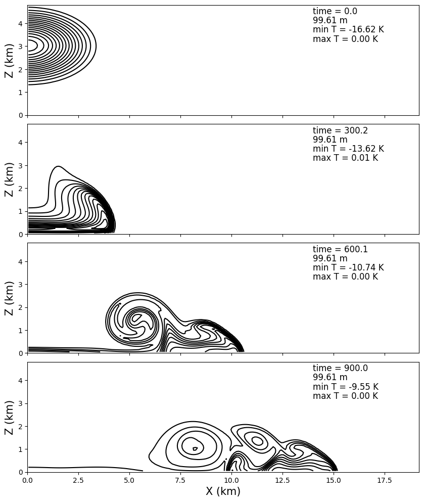
The maximum potential temperature anomaly should be zero because the motion is adiabatic and mimum potential temperature anomaly increases with time due to diffusion. The cold air spreads out as expected and develops rolling vortices. The result can be compared to Figure 3 of [2].